Current Research Interests and Publications
Finite Sample Bias of the Least Squares Estimator in an AR(p) Model: Estimation, Inference, Simulation and Examples.
Kerry Patterson
Department of Economics
The University of Reading
Abstract
This paper shows that the first order bias of least squares estimators of the coefficients of an AR(p) model is important for ‘typical’ macroeconomic time series and proposes a simple to apply method of bias reduction. Biases in individual coefficients often cumulate in the sum with far-reaching consequences for the cumulative impulse response function. This function, being nonlinear in the underlying coefficients, is particularly sensitive to biases when, as is often the case, the shocks are long-lived. Simulations and examples demonstrate some of the magnitudes involved.
Keywords: First order bias; long-run multiplier; autoregressive process.
JEL classification: C15; C22
(Forthcoming in Applied Economics)
Author’s address: K. D. Patterson, Department of Economics, University of Reading, Reading, Berks RG6 6AA, UK; 01189 318159/875123 ext 4439; fax 01189 750236; e-mail, b.l.sofocli@reading.ac.uk.
1. Introduction
It is well known that commonly used methods of estimation, for example least squares, Yule-Walker and maximum likelihood, of the coefficients in univariate p-th order autoregressive, AR, models exhibit a finite sample bias. Depending upon the true coefficient values, and sample size, this bias can be substantial and, as we show in this paper, have a marked effect not only on estimates of the individual AR coefficients but also on derived magnitudes of economic interest such as the impulse responses and long-run multiplier. The, latter being a non-linear function of the sum of the AR coefficients, q , it is particularly sensitive to small variations in estimated q when the generating process though stationary has a root close to the unit circle. Thus, correcting a ‘small’ bias in an estimate of q can have a pronounced effect on the long-run multiplier. One feature of finite sample bias not adequately considered previously is the way that apparently small biases in the individual AR coefficient estimates cumulate, often in a reinforcing rather than offsetting manner, in the estimate of the sum. Yet although bias reduction methods exist, they are rarely applied in practical examples. By offering a simple to compute (first order) bias adjusted estimator together with appropriate covariance matrix, this paper hopes to encourage a more routine assessment of bias reduction.
In an AR(1) model with known or unknown mean, estimated by least squares, Marriott and Pope (1954) and Kendall (1954) derived an expression for the O(1/T) bias, usually referred to as first order bias from the power on the sample size, T. First order bias tends to 0 as T ® ¥ . Implicit in the Mariott, Pope and Kendall approach was an adjustment that could reduce total bias by removing first order bias. However, the expression for first order bias depends upon the usually unknown true value of the AR coefficient, and overcoming this problem awaited Orcutt and Winokur (1969) who showed how to obtain a feasible estimator for the AR(1) model in which only higher order bias remained. Development of the MPK approach to more realistic higher order AR models was slow, related developments being made by Bhansali (1981), Tjøstheim and Paulsen (1983), Tanaka (1984), Pantula and Fuller (1985), Yamamoto and Kunitomo (1984), Kunitomo and Yamamoto (1985) and Cordeiro and Klein (1994).
The general structure of first order bias in the least squares estimator was revealed by Shaman and Stine (1988) and Stine and Shaman (1989), although an explicit first order bias adjusted, FOBA, estimator was not developed. We show how to generalise the Orcutt and Winokur procedure to the AR(p) model providing both a FOBA least squares estimator and associated covariance matrix. A simulation study shows that removal of first order bias is very effective in the overall reduction of finite sample bias at points in the parameter space likely to occur in practice. As the adjusted estimator and its covariance matrix are simple to compute this should encourage routine application of the method. Two examples, the first using the long-short spread on zero coupon U.S treasury bills/bonds and the second on the unemployment rate, illustrate some additional points.
This paper is organised as follows. Section 2 considers the impact of bias on estimates of the impulse response function and the long-run multiplier. Section 3 shows that the first order bias in least squares estimation is likely to be important for typical macroeconomic series. Section 4 shows how to obtain an estimator, covariance matrix and t statistics, based on removing the first order bias in the least squares estimator. Section 5 reports the results of some simulation experiments designed to assess the importance of first order bias relative to total bias. Section 6 considers some issues arising from two empirical examples and section 7 contains some concluding remarks. An appendix gives the first order bias adjusted estimators for AR(1) to AR(4) models.
2. The impact of biases on the impulse response function
We consider the stationary AR(p) model. That is:
![]() = m +
= m + ![]() +
+ ![]() (1) =
(1) = ![]() +
+ ![]() +
+ ![]() (2)
(2)
The error terms ![]() are iid with zero mean and constant variance. The least squares, LS, estimator of
are iid with zero mean and constant variance. The least squares, LS, estimator of ![]() = (1,
= (1, ![]() in (1) is
in (1) is ![]() = (1,
= (1, ![]() , where the elements of the estimated covariance matrix R are:
, where the elements of the estimated covariance matrix R are:
![]() =
= ![]() for i, j = 1, 2, ..., p (3)
for i, j = 1, 2, ..., p (3)
Where ![]() =
= ![]() and r = (
and r = (![]() , ...,
, ..., ![]() . In section 4 below we define
. In section 4 below we define ![]() (not italicised) just to contain the p unknown elements of
(not italicised) just to contain the p unknown elements of ![]() , so that
, so that ![]() =
= ![]() .
.
The extent of first order bias in the LS stimator is considered in section 3, and a simple and effective method of bias reduction is dealt with in section 4; here we consider the impact of bias on the long-run multiplier, which is the limit of the cumulative impulse response function, and the impulse responses.
It is useful to represent the information in an AR(p) model through its infinite moving average representation, which provides both the implied infinite sequence of lag weights and the impulse response function. From (2)
![]() (1
(1 ![]() = m (1
= m (1 ![]() +
+ ![]() (4)
(4)
and assuming stationarity then
![]() = m + w(L)
= m + w(L)![]() (5)
(5)
where w(L) º ![]() = (1
= (1![]() ,
, ![]() = 1. For low orders of p, the lag weights can be derived analytically by solving w(L)a (L) = 1 where a (L) º (1
= 1. For low orders of p, the lag weights can be derived analytically by solving w(L)a (L) = 1 where a (L) º (1![]() . The s-period cumulative response to a one-off one unit shock is given by
. The s-period cumulative response to a one-off one unit shock is given by ![]() , which graphed against s = 0, ..., ¥ , is the cumulative impulse response, CIR, function. The long-run effect is given by f º
, which graphed against s = 0, ..., ¥ , is the cumulative impulse response, CIR, function. The long-run effect is given by f º ![]() = (1
= (1![]() , where q º
, where q º ![]() and f is usually referred to as the long-run multiplier. In the AR(1) case, w(L) = 1 +
and f is usually referred to as the long-run multiplier. In the AR(1) case, w(L) = 1 + ![]() =
= ![]() = (1
= (1![]() and
and ![]() =
= ![]() .
.
Even if the bias in estimating individual coefficients is slight, if reinforcing it can accumulate in estimating q and have a devastating effect on the estimate of ![]() . Since macroeconomic time series are characterised by long memory, typically q is close to 1, with the implication that even a relatively small bias in estimating q is magnified in estimating
. Since macroeconomic time series are characterised by long memory, typically q is close to 1, with the implication that even a relatively small bias in estimating q is magnified in estimating ![]() . To illustrate assume that higher order bias is 0, then E{
. To illustrate assume that higher order bias is 0, then E{![]() } = q + b where b is the sum of first order biases in estimating
} = q + b where b is the sum of first order biases in estimating ![]() , and define the long run multiplier at the expected value of
, and define the long run multiplier at the expected value of ![]() as
as ![]() º (
º (![]() . Then
. Then
![]() =
= ![]() =
= ![]() (6)
(6)
Therefore
![]() –
– ![]() =
= ![]() (7)
(7)
The implied error in estimating the long-run multiplier at the expected value of ![]() is very sensitive to (1 – q ), especially through
is very sensitive to (1 – q ), especially through ![]() for q ‘close’ to 1; for example, suppose q = 0.9, implying
for q ‘close’ to 1; for example, suppose q = 0.9, implying ![]() = 10, and there is a 5% bias in
= 10, and there is a 5% bias in ![]() , then
, then ![]() –
– ![]() = –0.045/(0.01 + 0.0045) = –3.103, that is a –31.03% error in estimating
= –0.045/(0.01 + 0.0045) = –3.103, that is a –31.03% error in estimating ![]() .
.
Not only is the long run impact distorted by a small bias in estimating q , the complete time profile of the response is also affected. For example, consider the AR(1) model then, with unknown mean, the first order bias in the least squares estimator of ![]() is –(1 +3
is –(1 +3![]() )/T. With
)/T. With ![]() = 0.9 and T = 100, the first order bias is 0.037 or 4.111% of the true value. Assuming no higher order bias the expected value of
= 0.9 and T = 100, the first order bias is 0.037 or 4.111% of the true value. Assuming no higher order bias the expected value of ![]() (=
(= ![]() ) is 0.9 – 0.037 = 0.863. Given a one-off one-unit shock at time t, the impulse response at time t + h is
) is 0.9 – 0.037 = 0.863. Given a one-off one-unit shock at time t, the impulse response at time t + h is ![]() whereas the estimated impact is
whereas the estimated impact is ![]() . For h = 10 and
. For h = 10 and ![]() = 0.9 this is 0.3487, whereas for
= 0.9 this is 0.3487, whereas for ![]() = 0.863 it is 0.229. The ratio of the latter to the former is 0.657, so that an apparently small bias quickly cumulates through the nonlinear impact response function and the correct impact is underestimated by a factor of nearly 35% after 10 periods. Another aspect of the same problem is that the estimated half-life of the shock is 6.58 periods for
= 0.863 it is 0.229. The ratio of the latter to the former is 0.657, so that an apparently small bias quickly cumulates through the nonlinear impact response function and the correct impact is underestimated by a factor of nearly 35% after 10 periods. Another aspect of the same problem is that the estimated half-life of the shock is 6.58 periods for ![]() = 0.9 but only 4.70 periods for
= 0.9 but only 4.70 periods for ![]() = 0.863. This problem is accentuated, becoming quite extreme, as
= 0.863. This problem is accentuated, becoming quite extreme, as ![]() , or more generally q , ® 1.
, or more generally q , ® 1.
Evaluating the error in estimating ![]() as
as ![]() –
– ![]() is sensible because it mirrors what is done in practice, that is obtain an estimate of q and substitute that estimate into the expression for the calculation of
is sensible because it mirrors what is done in practice, that is obtain an estimate of q and substitute that estimate into the expression for the calculation of ![]() . Without bias adjustments to the LS estimator, and assuming higher order bias is zero, we cannot do better than use q + b, hence a relevant question is: what is the error when we do this? We could also evaluate the bias in estimating
. Without bias adjustments to the LS estimator, and assuming higher order bias is zero, we cannot do better than use q + b, hence a relevant question is: what is the error when we do this? We could also evaluate the bias in estimating ![]() by
by ![]() º
º ![]() , where the bias is E(
, where the bias is E(![]() ) -
) - ![]() . In general E(
. In general E(![]() ) ¹
) ¹ ![]() because
because ![]() is a nonlinear function of
is a nonlinear function of ![]() , say f(
, say f(![]() ). Provided f(
). Provided f(![]() ) is a convex function then from Jensen’s inequality, (see, for example, Rao (1973)), E[f(
) is a convex function then from Jensen’s inequality, (see, for example, Rao (1973)), E[f(![]() )] ³ f[E(
)] ³ f[E(![]() )]; applied here this states that E(
)]; applied here this states that E(![]() ) ³
) ³ ![]() , which may, therefore, place E(
, which may, therefore, place E(![]() ) closer to
) closer to ![]() . Note, however, that f(
. Note, however, that f(![]() ) is not everywhere a convex function. The second derivative of f(
) is not everywhere a convex function. The second derivative of f(![]() ) w.r.t
) w.r.t ![]() is 2
is 2![]() and positivity requires
and positivity requires ![]() < 1. Values of
< 1. Values of ![]() > 1 are possible even if q < 1, and when
> 1 are possible even if q < 1, and when ![]() crosses the unit boundary
crosses the unit boundary ![]() switches from large positive to negative. A more robust measure than the mean of the distribution of
switches from large positive to negative. A more robust measure than the mean of the distribution of ![]() is the median, and that is also reported below in section 5.
is the median, and that is also reported below in section 5.
3. Bias in least squares estimation
Shaman and Stine (1988) and Stine and Shaman (1989) derived expressions of the bias to order 1/T, the first order bias, of the LS estimator in an AR(p) model and showed that certain very particular finite order models are unbiased. These are projections of a unique (up to scale) infinite order process: the fixed point for a particular model order. If the time series is not generated by this process, the bias of the LS estimator pulls the estimator closer to the fixed point coefficients. We briefly outline this approach and then show how it can be operationalised. Whilst the method is illustrated with some low order examples, this is purely for expositional purposes as the method can be applied quite generally.
The DGP is assumed to be the stationary AR(p) model given by (2). Expressions for bias reduction depend upon whether m is known or unknown. Because in most practical situations m is unknown we concentrate on that case here. Shaman and Stine (1988) and Stine and Shaman (1989) show that, when m is unknown, then:
bias(![]() ) º E(
) º E(![]() ) – a = –
) – a = – ![]() + o(1/T) (8)
+ o(1/T) (8)
Where ![]() =
= ![]() ,
, ![]() is a (p + 1) x (p +1) matrix of known coefficients and o(1/T) indicates terms of higher order than 1/T. Interpretation of (8) is as follows. The bias in the least squares estimator
is a (p + 1) x (p +1) matrix of known coefficients and o(1/T) indicates terms of higher order than 1/T. Interpretation of (8) is as follows. The bias in the least squares estimator ![]() is decomposed into first order bias given by –
is decomposed into first order bias given by –![]() and terms of higher order, for example functions of 1/
and terms of higher order, for example functions of 1/![]() , 1/
, 1/![]() and so on, indicated by o(1/T).
and so on, indicated by o(1/T).
To construct the matrix ![]() , first calculate the following 3 matrices:
, first calculate the following 3 matrices: ![]() ,
, ![]() and
and ![]() . Where
. Where ![]() = diag(0, 1, ..., p);
= diag(0, 1, ..., p); ![]() has columns which are based on the column vectors
has columns which are based on the column vectors ![]() and
and ![]() ; the elements of
; the elements of ![]() and
and ![]() are 0 apart from a 1 in rows j + 3, j + 5, p + 1 – j for
are 0 apart from a 1 in rows j + 3, j + 5, p + 1 – j for ![]() , and rows j + 2, j + 4, p + 1 – j for
, and rows j + 2, j + 4, p + 1 – j for ![]() . When p is even
. When p is even ![]() = [–
= [–![]() ,–
,–![]() , ..., -
, ..., -![]() ,...,
,..., ![]() ,
, ![]() ] where k = (p/2) – 1. When p is odd
] where k = (p/2) – 1. When p is odd ![]() = [–
= [–![]() , –
, –![]() , ..., –
, ..., –![]() , 0 ,
, 0 , ![]() , ...,
, ..., ![]() ,
, ![]() ,
, ![]() ). The (i, j) element of
). The (i, j) element of ![]() is –1 for j < i £ r and 1 for r < i £ j, where r = p – j +2, and 0 elsewhere. Next sum
is –1 for j < i £ r and 1 for r < i £ j, where r = p – j +2, and 0 elsewhere. Next sum ![]() ,
, ![]() and
and ![]() , and then change the sign of elements in the first column; the resulting matrix is
, and then change the sign of elements in the first column; the resulting matrix is ![]() .
.
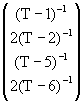
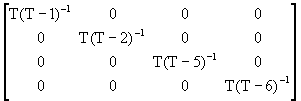
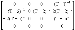
An example may help to show how the bias expressions are calculated. With p = 4, we have:
(![]() +
+ ![]() +
+ ![]() )
)
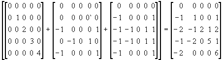 (9)
(9)
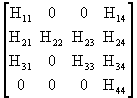
and, therefore, with a change of sign in the first column
![]()
![]()
 (10)
(10)
Thus, for example, the first order bias in estimating ![]() by least squares is –(1 +
by least squares is –(1 + ![]() +
+ ![]() )/T.
)/T.
Next it is helpful to define the bias for each ![]() i = 1, ..., p. Let
i = 1, ..., p. Let ![]() be the i-th row of –
be the i-th row of –![]() /T, then the bias in estimating
/T, then the bias in estimating ![]() is the scalar
is the scalar ![]() a . The bias vector is the p x 1 column vector with
a . The bias vector is the p x 1 column vector with ![]() a in the i-th element.
a in the i-th element.
Often in economic analysis q and ![]() are of greater interest than the individual lag coefficients. The least squares estimator of the long-run coefficient is
are of greater interest than the individual lag coefficients. The least squares estimator of the long-run coefficient is ![]() º
º ![]() with first order bias b =
with first order bias b = ![]() , which is the sum of the elements in the bias vector. At a fixed point in the parameter space of the DGP, the LS bias for the individual coefficients is zero, otherwise it is nonzero. Table 1 gives the first order bias, b, for the LS estimator of the long-run coefficient in the AR(p) models, p = 1, ..., 4, and the zero bias fixed points.
, which is the sum of the elements in the bias vector. At a fixed point in the parameter space of the DGP, the LS bias for the individual coefficients is zero, otherwise it is nonzero. Table 1 gives the first order bias, b, for the LS estimator of the long-run coefficient in the AR(p) models, p = 1, ..., 4, and the zero bias fixed points.
Table 1. AR coefficients corresponding to zero first order bias
Total first order bias in ![]() Zero bias coefficients
Zero bias coefficients
AR(1): –(1 + 3![]() )/T
)/T ![]() = –
= –![]()
AR(2): –(3 + ![]() + 5
+ 5![]() )/T
)/T ![]() = –0.5,
= –0.5, ![]() = –0.5
= –0.5
AR(3): –(4 + 4![]() + 8
+ 8![]() )/T
)/T ![]() = –0.6,
= –0.6, ![]() = –0.6,
= –0.6, ![]() = –0.2
= –0.2
AR(4): –(6 – 2![]() + 2
+ 2![]() + 6
+ 6![]() + 10
+ 10![]() )/T
)/T ![]() = –
= –![]() ,
, ![]() = –0.8,
= –0.8, ![]() = –0.4,
= –0.4, ![]() = –
= –![]()
A question of interest in this context is what do processes generated by the zero bias coefficients in Table 1 look like and, in particular, do they look like typical (macro)economic processes?
The implied lag weights for the fixed points of the AR(1) to AR(4) models are shown in Figures 1a – 1d. The different AR models show a very similar pattern with, in each case, a mixture of negative and positive weights implying a non-monotonic CIR function. This pattern does not appear typical of stationary AR models fitted to macroeconomic time series. For comparison we selected typical, or stylised, AR coefficients from the estimates of the Nelson and Plosser (1982) data set of 14 macroeconomic time series variously spanning 1860 to 1988. These were as follows. AR(2) coefficients: ![]() = 1.25,
= 1.25, ![]() = –0.35; AR(3) coefficients:
= –0.35; AR(3) coefficients: ![]() = 1.3,
= 1.3, ![]() = –0.5,
= –0.5, ![]() = 0.1; AR(4) coefficients:
= 0.1; AR(4) coefficients: ![]() = 1.2,
= 1.2, ![]() = –0.55,
= –0.55, ![]() = 0.4,
= 0.4, ![]() = –0.15; in addition, for an AR(1) model we chose
= –0.15; in addition, for an AR(1) model we chose ![]() = 0.9 as typical of the simplest model. In each case q = 0.9 and f = 10, these latter capturing the long but not infinite memory typical of macroeconomic time series. Andrews (1994) notes of estimates using the Schotman and van Dijk (1991) extension of Nelson and Plosser’s original sample that "Most of the real variables – including real gross national product (GNP), real per capita GNP, industrial production, and employment have a [here q is a , my clarification] estimates in the range .86 to .91 ...". The response functions implied by this choice are also shown on Figures 1a to 1d. In contrast to the zero bias case the adjustment to a shock is much smoother for the stylised coefficients.
= 0.9 as typical of the simplest model. In each case q = 0.9 and f = 10, these latter capturing the long but not infinite memory typical of macroeconomic time series. Andrews (1994) notes of estimates using the Schotman and van Dijk (1991) extension of Nelson and Plosser’s original sample that "Most of the real variables – including real gross national product (GNP), real per capita GNP, industrial production, and employment have a [here q is a , my clarification] estimates in the range .86 to .91 ...". The response functions implied by this choice are also shown on Figures 1a to 1d. In contrast to the zero bias case the adjustment to a shock is much smoother for the stylised coefficients.
Using the stylised AR(p) coefficients as the true values, we calculated the total first order bias in estimating the long-run coefficient q and the error, ![]() –
– ![]() , in the implied long-run multiplier for various sample sizes. In practice higher order biases will also be present and a simulation study reported in section 5 provides evidence on the extent of such biases. The results are reported in Table 2, where the table entries are the %bias in estimating q and the implied error in estimating f , respectively. The broad pattern of first order bias is similar across the 4 AR(p) specifications, with the bias always negative, that is q and f are underestimated. With the smaller sample sizes the first order bias is large, resulting in substantial underestimates of the long-run multiplier. For example, in the AR(2) model where f = 10, then with first order bias the estimated f for T = 25 is 5, for T = 100 it is 8, and even with a relatively large sample size of T = 200 it is 8.88, so that the error is just over –11% of the true value.
, in the implied long-run multiplier for various sample sizes. In practice higher order biases will also be present and a simulation study reported in section 5 provides evidence on the extent of such biases. The results are reported in Table 2, where the table entries are the %bias in estimating q and the implied error in estimating f , respectively. The broad pattern of first order bias is similar across the 4 AR(p) specifications, with the bias always negative, that is q and f are underestimated. With the smaller sample sizes the first order bias is large, resulting in substantial underestimates of the long-run multiplier. For example, in the AR(2) model where f = 10, then with first order bias the estimated f for T = 25 is 5, for T = 100 it is 8, and even with a relatively large sample size of T = 200 it is 8.88, so that the error is just over –11% of the true value.
Table 2. First order bias in estimating q and implied error for f in ‘typical’ AR(p) models
|
T |
25 |
50 |
75 |
100 |
200 |
|
AR(1) |
|
|
|
|
|
|
q %bias |
–16.44 |
–8.22 |
–5.48 |
–4.11 |
–2.05 |
|
f %error |
–59.68 |
–42.53 |
–33.04 |
–27.01 |
–15.62 |
|
AR(2) |
|
|
|
|
|
|
q %bias |
–11.11 |
–5.56 |
–3.70 |
–2.78 |
–1.39 |
|
f %error |
–50.00 |
–33.33 |
–25.00 |
–20.00 |
–11.12 |
|
AR(3) |
|
|
|
|
|
|
q %bias |
–12.44 |
–6.22 |
–4.15 |
–3.11 |
–1.56 |
|
f %error |
–52.83 |
–35.90 |
–27.18 |
–21.88 |
–12.28 |
|
AR(4) |
|
|
|
|
|
|
q %bias |
–15.11 |
–7.55 |
–5.04 |
–3.78 |
–1.89 |
|
f %error |
–57.63 |
–40.48 |
–31.20 |
–25.37 |
–14.53 |
Notes: table entries are first order bias for ![]() and implied error for
and implied error for ![]() as % of the true coefficient. The AR coefficients are as follows: AR(1),
as % of the true coefficient. The AR coefficients are as follows: AR(1), ![]() = 0.9; AR(2),
= 0.9; AR(2), ![]() = 1.25,
= 1.25, ![]() = –0.35; AR(3),
= –0.35; AR(3), ![]() = 1.3,
= 1.3, ![]() = –0.5,
= –0.5, ![]() = 0.1; AR(4),
= 0.1; AR(4), ![]() = 1.2,
= 1.2, ![]() = –0.55,
= –0.55, ![]() = 0.4,
= 0.4, ![]() = –0.15. The sum of first order bias is calculated as shown in Table 1.
= –0.15. The sum of first order bias is calculated as shown in Table 1.
4. Bias Reduction
In this section we derive an operational first order bias adjustment to the least squares estimator ![]() of
of ![]() . The resulting estimator is denoted
. The resulting estimator is denoted ![]() and referred to as the FOBALS estimator (first order bias adjusted least squares). Corresponding adjustments are also given to obtain the correct estimated standard errors.
and referred to as the FOBALS estimator (first order bias adjusted least squares). Corresponding adjustments are also given to obtain the correct estimated standard errors.
The problem with the implied first order bias adjustments given in section 3 is that they are not operational because they depend on the unknown true values of the AR coefficients. Consider this problem in the AR(1) case where, apart from higher order terms, E{![]() } =
} = ![]() – (1 + 3
– (1 + 3![]() )/T but
)/T but ![]() is unknown. One possible solution is to use any consistent estimator of
is unknown. One possible solution is to use any consistent estimator of ![]() , unadjusted least squares being an obvious choice so that the revised estimator is
, unadjusted least squares being an obvious choice so that the revised estimator is ![]() + (1 + 3
+ (1 + 3![]() )/T. However, because
)/T. However, because ![]() tends to underestimate
tends to underestimate ![]() the bias will also be underestimated. The problem is pervasive whatever the order of the AR model. Generalising a procedure due to Orcutt and Winokur (1969) it is possible to do better than this. In the AR(1) case substitute
the bias will also be underestimated. The problem is pervasive whatever the order of the AR model. Generalising a procedure due to Orcutt and Winokur (1969) it is possible to do better than this. In the AR(1) case substitute ![]() for E{
for E{![]() } and solve for the unknown
} and solve for the unknown ![]() , which is considered as an estimator and denoted
, which is considered as an estimator and denoted ![]() ; this gives
; this gives ![]() =
= ![]() T/(T – 3) + 1/(T – 3). This procedure completely eliminates the first order bias for
T/(T – 3) + 1/(T – 3). This procedure completely eliminates the first order bias for ![]() taking its expected value.
taking its expected value.
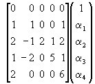
The general form of the solution, which does not appear to have been given before, is as follows. First it is convenient to define ![]() (not italicised) just to contain estimators of the p unknown AR coefficients; that is
(not italicised) just to contain estimators of the p unknown AR coefficients; that is ![]() = (
= (![]() , ...,
, ..., ![]() and, correspondingly,
and, correspondingly, ![]() = (
= (![]() , ...,
, ..., ![]() . There are two steps in the derivation of the adjusted estimator. In the first step substitute
. There are two steps in the derivation of the adjusted estimator. In the first step substitute ![]() for E{
for E{![]() } in E{
} in E{![]() } -
} - ![]() =
= ![]() a , where
a , where ![]() a is the i-th element of the bias vector defined in section 3 and will depend upon the order of the AR(p) model – see, for example, (10) – and then collect terms. This gives an equation system that can be expressed in the following general form (the second step):
a is the i-th element of the bias vector defined in section 3 and will depend upon the order of the AR(p) model – see, for example, (10) – and then collect terms. This gives an equation system that can be expressed in the following general form (the second step):
![]() = t +
= t + ![]() +
+ ![]() (11)
(11)
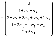
Solving for ![]() we obtain:
we obtain:
![]() =
= ![]() t +
t + ![]()
![]() (12a)
(12a)
say ![]() = k + H
= k + H![]() (12b)
(12b)
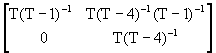
where H º ![]()
![]() . The parameters in t ,
. The parameters in t , ![]() and
and ![]() are defined following the first step and depend upon the parameters in
are defined following the first step and depend upon the parameters in ![]() . The system (11) can either be solved as in (12) or by reordering
. The system (11) can either be solved as in (12) or by reordering ![]() into a lower triangular matrix and then exploiting the recursive structure of the solution starting with
into a lower triangular matrix and then exploiting the recursive structure of the solution starting with ![]() . As the matrix H is required to compute the appropriate standard errors it is probably more convenient to work with (12), especially for higher order AR models. An appendix gives explicit solutions for the AR(2), AR(3) and AR(4) models. By construction E{
. As the matrix H is required to compute the appropriate standard errors it is probably more convenient to work with (12), especially for higher order AR models. An appendix gives explicit solutions for the AR(2), AR(3) and AR(4) models. By construction E{![]() } = a + o(1/T), so that first order biases are eliminated.
} = a + o(1/T), so that first order biases are eliminated.
The estimated standard errors of the bias adjusted estimators are the square roots of the diagonal elements of the variance-covariance matrix of ![]() , Var(
, Var(![]() ), where Var(
), where Var(![]() ) = H[Var(
) = H[Var(![]() )]
)]![]() . As unadjusted least squares produces minimum variance estimators the cost of removing first order bias in expectation is an increase in variance, although it does not necessarily follow that the t statistics for individual coefficients will decline. A commonly used criterion for comparing different estimators, at least one of which is biased, is root mean square error, rmse, which weights equally squared bias and variance; hence, a comparison in terms of rmse will not necessarily favour the bias adjusted estimator.
. As unadjusted least squares produces minimum variance estimators the cost of removing first order bias in expectation is an increase in variance, although it does not necessarily follow that the t statistics for individual coefficients will decline. A commonly used criterion for comparing different estimators, at least one of which is biased, is root mean square error, rmse, which weights equally squared bias and variance; hence, a comparison in terms of rmse will not necessarily favour the bias adjusted estimator.
5. Simulation results
The aim of the simulation experiments is to illustrate and assess the gain from adjusting LS estimators for first order bias. There are several aspects to this assessment. Whilst first order bias is only known if the AR coefficients are known and, generally, the latter are not known, the method of estimation described above removes first order bias leaving only higher order bias. Thus, total bias can be decomposed into first order and higher order biases. Whilst we anticipate that a large part of the total finite sample bias is accounted for by the first order bias, it will be useful to know how this works in typical cases. The second aspect of interest concerns the effect of the bias on estimating the long-run coefficients q and f ; as noted above apparently small biases in estimating the individual AR coefficients may be translated into a substantial bias in estimating q and a potentially very substantial error in estimating f .
There are four tables, one for each AR(p) model – see Tables 3 to 6. The DGP is given by (2), that is
![]() =
= ![]() +
+ ![]() +
+ ![]() ,
, ![]() ~ niid(0, 1)
~ niid(0, 1)
The design parameters for the four AR(p) models, p = 1, ..., 4, were those used in Table 1 based on typical AR coefficients; throughout q = 0.9, so that f = 10, reflecting the high persistence found in macroeconomic time series and m = 0.1. There are 50,000 replications in each experiment; effective sample sizes are T = 50, 100, 200 with the first 150 replications discarded in each case.
In each table, and for each AR coefficient, the first row entries refer to the theoretical first order bias for different sample sizes, expressed as a percentage of the absolute value of the true coefficient; these rows are headed ![]() FOB. The second and third rows, in each case, give the mean bias over 50000 replications for
FOB. The second and third rows, in each case, give the mean bias over 50000 replications for ![]() and
and ![]() , respectively, expressed as a percentage of the absolute value of the true coefficient.
, respectively, expressed as a percentage of the absolute value of the true coefficient. ![]() and
and ![]() are, respectively, the least squares and (first) order bias adjusted estimators. For a positive coefficient a negative bias indicates that the coefficient is underestimated; for example, if
are, respectively, the least squares and (first) order bias adjusted estimators. For a positive coefficient a negative bias indicates that the coefficient is underestimated; for example, if ![]() = 1.2 and
= 1.2 and ![]() = 1.08 then the %mean bias is 100(1.08 – 1.2)/1.2 = –10%. For a negative coefficient a positive bias indicates that the coefficient is underestimated in absolute value; for example, if
= 1.08 then the %mean bias is 100(1.08 – 1.2)/1.2 = –10%. For a negative coefficient a positive bias indicates that the coefficient is underestimated in absolute value; for example, if ![]() = –0.55 and
= –0.55 and ![]() = –0.495 then the %mean bias is 100(–0.495 –(– 0.55))/0.55 = 10%. Similar row entries, that is %mean bias, are given for q and their respective LS and FOBALS estimators. The next set of three row entries is as follows. The first of these is the %mean error in the implied value of
= –0.495 then the %mean bias is 100(–0.495 –(– 0.55))/0.55 = 10%. Similar row entries, that is %mean bias, are given for q and their respective LS and FOBALS estimators. The next set of three row entries is as follows. The first of these is the %mean error in the implied value of ![]() assuming just first order bias in
assuming just first order bias in ![]() (these are from Table 1), this row is denoted
(these are from Table 1), this row is denoted ![]() FOB. Then, following earlier notation, the entries for
FOB. Then, following earlier notation, the entries for ![]() and
and ![]() give the % error, and then the actual values, for
give the % error, and then the actual values, for ![]() and
and ![]() evaluated at the means of
evaluated at the means of ![]() and
and ![]() , respectively. Also, following
, respectively. Also, following ![]() and
and ![]() , the median values of the empirical distributions of
, the median values of the empirical distributions of ![]() and
and ![]() are reported.
are reported.
In addition, in the second column for each sample size, there is a comparison of rmse. Specifically, the table entry is the ratio of the rmse of the LS estimator to the FOBALS estimator for the individual coefficients and their sum. Recall that the rmse is the square root of the variance plus the squared bias, and the variance for the FOBALS estimator cannot be less than that for the LS estimator. Hence, the rmse ratio indicates whether, with equal weights for squared bias and variance, the reduction in bias outweighs the increase in variance – if so the ratio will be greater than 1.
In interpreting the results note that the total least squares bias, that is the table entry for ![]() , is approximately the sum of the first order bias and the bias using
, is approximately the sum of the first order bias and the bias using ![]() . Hence, the latter is the higher order bias remaining after the first order bias has been removed.
. Hence, the latter is the higher order bias remaining after the first order bias has been removed.
The results for the simplest model, that is AR(1), set the scene for the remaining models. In the AR(1) model with T = 50, there is a first order bias of –8.222% in estimating ![]() by least squares; the second row entry shows that this is most of the total least squares bias of –8.969%. The first order bias is removed using the FOBALS estimator,
by least squares; the second row entry shows that this is most of the total least squares bias of –8.969%. The first order bias is removed using the FOBALS estimator, ![]() , to leave a bias, attributable to terms of higher order than the first, of –0.794%. The mean estimates of
, to leave a bias, attributable to terms of higher order than the first, of –0.794%. The mean estimates of ![]() and
and ![]() are 0.819 and 0.893, respectively, with a rmse ratio of 1.242 indicating a substantial benefit to using
are 0.819 and 0.893, respectively, with a rmse ratio of 1.242 indicating a substantial benefit to using ![]() . The implied estimates for the long-run multiplier are
. The implied estimates for the long-run multiplier are ![]() = 5.533 and
= 5.533 and ![]() = 9.332. The former is a substantial underestimate of the correct value of 10.0. The medians of the empirical distributions of
= 9.332. The former is a substantial underestimate of the correct value of 10.0. The medians of the empirical distributions of ![]() and
and ![]() are 6.085 and 8.642, respectively, which is only slightly less favourable to the FOBALS estimator.
are 6.085 and 8.642, respectively, which is only slightly less favourable to the FOBALS estimator.
Even with a moderate sample size of T = 100, considerable problems remain for LS estimation. ![]() again dominates
again dominates ![]() with higher order bias slight relative to total bias and a 19% increase in rmse using
with higher order bias slight relative to total bias and a 19% increase in rmse using ![]() rather than
rather than ![]() . As for estimating
. As for estimating ![]() , the mean error of –4.419% for
, the mean error of –4.419% for ![]() is deceptive since it implies
is deceptive since it implies ![]() = 7.154, which is well below the true value. Using
= 7.154, which is well below the true value. Using ![]() results in a mean error of –0.318% and
results in a mean error of –0.318% and ![]() = 9.722. The corresponding medians of
= 9.722. The corresponding medians of ![]() and
and ![]() are 7.618 and 10.555, again favouring the bias adjusted estimator. The impact of an apparently small bias in estimating q on the estimation of
are 7.618 and 10.555, again favouring the bias adjusted estimator. The impact of an apparently small bias in estimating q on the estimation of ![]() was demonstrated in (6) and (7), and is very effectively shown with the simulation results for T = 200. There is a –2.34% mean bias in estimating q by least squares, but this implies
was demonstrated in (6) and (7), and is very effectively shown with the simulation results for T = 200. There is a –2.34% mean bias in estimating q by least squares, but this implies![]() = 8.390, an error of –16.11%; in contrast
= 8.390, an error of –16.11%; in contrast ![]() = 9.929. The medians of
= 9.929. The medians of ![]() and
and ![]() are 8.725 and 10.412, so
are 8.725 and 10.412, so ![]() is also favoured on this criterion.
is also favoured on this criterion.
The AR(4) case is of particular interest because if frequently occurs in practice. The first order biases for the individual coefficients are deceptively slight. For example, with T = 50, where the true coefficient is given in brackets, they are: -0.041 (1.2); 0.004 (–0.55); -0.009 (0.4); -0.022 (–0.15). The net effect of the first order bias on q is negative with a sum equal to –0.068 relative to 0.9, that is –7.556%, and implied f equal to 5.952. The mean of ![]() is 0.8196 so that the mean total LS bias in estimating q by
is 0.8196 so that the mean total LS bias in estimating q by ![]() is -8.935%; the mean of the bias adjusted estimator,
is -8.935%; the mean of the bias adjusted estimator, ![]() , is 0.888, a mean bias, attributable to higher order terms, of 0.012 = –1.356%. Whilst only one of the rmse ratios for the individual coefficients is above 1, the rmse ratio for the sum of the AR coefficients is well above 1, indicating that on this criterion the bias reduction is worth having. The implied values of
, is 0.888, a mean bias, attributable to higher order terms, of 0.012 = –1.356%. Whilst only one of the rmse ratios for the individual coefficients is above 1, the rmse ratio for the sum of the AR coefficients is well above 1, indicating that on this criterion the bias reduction is worth having. The implied values of ![]() and
and ![]() at the mean estimates of
at the mean estimates of ![]() and
and ![]() are
are ![]() = 5.542 and
= 5.542 and ![]() = 8.913, with medians of 6.148 and 8.428, respectively. The extent of the errors from least squares estimation of
= 8.913, with medians of 6.148 and 8.428, respectively. The extent of the errors from least squares estimation of ![]() must cast doubt on whether it is sensible to report this measure without some attempt at bias adjustment.
must cast doubt on whether it is sensible to report this measure without some attempt at bias adjustment.
As in the AR(1) case, although a larger sample size attenuates the effects of first and higher order bias, sizeable biases still remain, which may, in practical examples, have a marked effect on parameters of economic interest. For example, with AR(4) and T = 100 the mean bias of ![]() is –4.164% compared to –0.387% for
is –4.164% compared to –0.387% for ![]() , and a rmse ratio of 1.162. The implied long-run multipliers from these mean values are 7.274 and 9.664, respectively, with medians of KKKKK, respectively.
, and a rmse ratio of 1.162. The implied long-run multipliers from these mean values are 7.274 and 9.664, respectively, with medians of KKKKK, respectively.
The picture from the AR(2) and AR(3) models is similar to that for the AR(4) model. For T = 50 there is a bias of about 6 or 7% in estimating ![]() by least squares, of which less than l% point is due to higher order biases. Whilst the rmse ratio for the LS and FOBALS estimates is not uniformly above 1 for individual coefficients, it is noticeably above 1 in estimating the sum of the AR coefficients. The rmse is typically about 20% higher for the LS estimator when T = 50 reducing to about 9% with T = 200; hence, removing the first order bias generally offers useful gains in overall bias reduction and reduction in rmse. The implied values of
by least squares, of which less than l% point is due to higher order biases. Whilst the rmse ratio for the LS and FOBALS estimates is not uniformly above 1 for individual coefficients, it is noticeably above 1 in estimating the sum of the AR coefficients. The rmse is typically about 20% higher for the LS estimator when T = 50 reducing to about 9% with T = 200; hence, removing the first order bias generally offers useful gains in overall bias reduction and reduction in rmse. The implied values of ![]() at the mean of
at the mean of ![]() substantially underestimate
substantially underestimate ![]() , whereas much of this error is removed by using
, whereas much of this error is removed by using ![]() . A comparison in terms of the medians of the empirical distributions of
. A comparison in terms of the medians of the empirical distributions of ![]() and
and ![]() is only slightly less favourable. As in the AR(1) and AR(4) cases the LS estimate of
is only slightly less favourable. As in the AR(1) and AR(4) cases the LS estimate of ![]() has little to recommend it.
has little to recommend it.
Comparing different sample sizes, note that because the bias in ![]() is of higher order than first, it reduces faster than linearly and so proportionately more quickly than the bias in
is of higher order than first, it reduces faster than linearly and so proportionately more quickly than the bias in ![]() . A rough rule of thumb is that the bias in
. A rough rule of thumb is that the bias in ![]() reduces to about one-third from a doubling of the sample size; thus, quadrupling the sample size reduces the bias in
reduces to about one-third from a doubling of the sample size; thus, quadrupling the sample size reduces the bias in ![]() to about 1/9th of its initial value.
to about 1/9th of its initial value.
Table 3. AR(1): First order bias, LS bias, FOBALS bias; ![]() = 0.9
= 0.9
% mean bias/error
|
|
T = 50 |
rmse ratio |
T = 100 |
rmse ratio |
T = 200 |
rmse ratio |
|
|
–8.222 |
|
–4.111 |
|
–2.056 |
|
|
|
–8.969 |
1.242 |
–4.419 |
1.187 |
–2.134 |
1.165 |
|
|
–0.794 |
|
–0.318 |
|
–0.079 |
|
|
|
–42.530 5.747 |
|
–27.007 7.300 |
|
–15.612 8.439 |
|
|
|
–44.670 5.533 6.085 |
|
–28.455 7.154 7.618 |
|
–16.110 8.389 8.725 |
|
|
|
–6.680 9.332 8.642 |
|
–2.780 9.722 10.555 |
|
–0.710 9.929 10.412 |
|
Table 4. AR(2): First order bias, LS bias, FOBALS bias; ![]() = 1.25,
= 1.25, ![]() = –0.35
= –0.35
% mean bias/error
|
|
T = 50 |
rmse ratio |
T = 100 |
rmse ratio |
T = 200 |
rmse ratio |
|
|
–3.040 |
|
–1.520 |
|
–0.760 |
|
|
|
–3.662 |
1.047 |
–1.586 |
1.020 |
–0.775 |
1.010 |
|
|
–0.632 |
|
–0.067 |
|
–0.015 |
|
|
|
–3.428 |
|
–1.714 |
|
–0.857 |
|
|
|
–2.994 |
0.923 |
–1.923 |
0.963 |
–0.978 |
0.981 |
|
|
0.473 |
|
–0.217 |
|
–0.124 |
|
|
q %FOB |
–5.556 |
|
–2.778 |
|
–1.389 |
|
|
|
–6.256 |
1.199 |
–2.951 |
1.136 |
–1.457 |
1.087 |
|
|
–0.695 |
|
–0.178 |
|
–0.069 |
|
|
|
–33.334 6.666 |
|
–20.000 8.000 |
|
–11.111 8.888 |
|
|
|
–36.003 6.397 6.933 |
|
–20.983 7.902 8.307 |
|
–11.590 8.841 9.080 |
|
|
|
–5.882 9.412 9.831 |
|
-1.577 9.842 10.465 |
|
–0.618 9.938 10.248 |
|
Table 5. AR(3): First order bias, LS bias, FOBALS bias;![]() = 1.3,
= 1.3, ![]() = –0.5,
= –0.5, ![]() = 0.1
= 0.1
% mean bias/error
|
|
T = 50 |
r.m.s.e ratio |
T = 100 |
r.m.s.e ratio |
T = 200 |
r.m.s.e ratio |
|
|
|
–3.846 |
|
-1.923 |
|
–0.962 |
|
|
|
|
–4.553 |
1.037 |
–2.111 |
1.017 |
–0.983 |
1.007 |
|
|
|
–0.725 |
|
–0.191 |
|
–0.022 |
|
|
|
|
4.800 |
|
2.400 |
|
1.200 |
|
|
|
|
5.323 |
0.928 |
2.657 |
0.964 |
1.140 |
0.981 |
|
|
|
0.615 |
|
0.290 |
|
–0.061 |
|
|
|
|
–30.000 |
|
–15.000 |
|
–7.500 |
|
|
|
|
–31.238 |
0.922 |
–15.981 |
0.962 |
–7.669 |
0.981 |
|
|
|
–1.376 |
|
–1.033 |
|
–0.173 |
|
|
|
q FOB |
–6.222 |
|
–3.111 |
|
–1.555 |
|
|
|
|
–7.086 |
1.179 |
–3.339 |
1.136 |
–1.639 |
1.088 |
|
|
|
–0.861 |
|
–0.230 |
|
–0.085 |
|
|
|
|
–35.898 6.410 |
|
–21.875 7.813 |
|
–12.281 8.772 |
|
|
|
|
-38.940 6.106 6.673 |
|
–23.100 7.690 8.142 |
|
–12.870 8.713 8.986 |
|
|
|
|
-7.190 9.281 9.343 |
|
–2.030 9.797 10.511 |
|
-0.750 9.925 10.274 |
|
|
Table 6. AR(4): First order bias, LS bias, FOBALS bias; ![]() = 1.2,
= 1.2, ![]() = –0.55,
= –0.55, ![]() = 0.4,
= 0.4, ![]() = –0.15
= –0.15
% mean bias/error
|
|
T = 50 |
r.m.s.e ratio |
T = 100 |
r.m.s.e ratio |
T = 200 |
r.m.s.e ratio |
|
|
|
-3.417 |
|
-1.708 |
|
-0.858 |
|
|
|
|
-4.325 |
1.039 |
-1.941 |
1.017 |
-0.902 |
1.008 |
|
|
|
-0.927 |
|
-0.236 |
|
-0.049 |
|
|
|
|
0.727 |
|
0.364 |
|
0.182 |
|
|
|
|
0.903 |
0.956 |
0.394 |
0.988 |
0.127 |
0.989 |
|
|
|
0.216 |
|
0.034 |
|
-0.055 |
|
|
|
|
-2.250 |
|
-1.125 |
|
-0.563 |
|
|
|
|
-2.871 |
0.920 |
-1.218 |
0.960 |
-0.534 |
0.980 |
|
|
|
-0.566 |
|
-0.084 |
|
0.029 |
|
|
|
|
-14.667 |
|
-7.333 |
|
-3.667 |
|
|
|
|
-14.660 |
0.891 |
-7.647 |
0.946 |
-3.832 |
0.973 |
|
|
|
0.007 |
|
-0.336 |
|
-0.171 |
|
|
|
q FOB |
-7.556 |
|
-3.778 |
|
-1.889 |
|
|
|
|
-8.935 |
1.204 |
-4.164 |
1.162 |
-2.002 |
1.104 |
|
|
|
-1.356 |
|
-0.387 |
|
-0.113 |
|
|
|
|
-40.476 5.952 |
|
–25.374 7.463 |
|
-14.530 8.547 |
|
|
|
|
-44.572 5.542 6.148
|
|
-27.257 7.274 tba |
|
-15.267 8.473 tba |
|
|
|
|
-10.866 8.913 8.428 |
|
-3.363 9.664 tba |
|
-1.013 9.899 tba |
|
|
6. Examples
As section 5 was concerned with simulation experiments using stylised coefficients based on Nelson and Plosser’s study of 14 macroeconomic series, two different examples are used here in order to illustrate some other points. The first example is the long-short spread using data on zero coupon U.S Treasury bills and bonds. This example demonstrates relatively large changes in the estimated coefficients, for example a 17% difference between estimates of the sum of AR coefficients; but, because the process is far from the unit circle, estimates of the long-run multiplier remain ‘relatively’ robust. The second example illustrates a different case. Using quarterly data on the U.S unemployment rate, apparently relatively minor differences between estimates lead to a large change in estimates of the long-run multiplier.
6.i Spread Between U.S 1-Month Treasury Bills and 10-Year Treasury Bonds
The data used here is annual for the period 1950 to 1993, a total of 44 observations, on the zero coupon yield on 1-month U.S Treasury bills, ![]() , and 10 year U.S Treasury bonds,
, and 10 year U.S Treasury bonds, ![]() ; from these we define the long-short spread,
; from these we define the long-short spread, ![]() º
º ![]() –
– ![]() . An AR(2) model was fitted to this data. The preferred model was selected on the basis of: information criteria (AIC, SIC and Hannan-Quinn leading to the same choice); F and marginal t tests for simplification from AR(4), again leading to AR(2); and residuals free from serial correlation with a standard LM(4) test giving a marginal significance level of 93%.
. An AR(2) model was fitted to this data. The preferred model was selected on the basis of: information criteria (AIC, SIC and Hannan-Quinn leading to the same choice); F and marginal t tests for simplification from AR(4), again leading to AR(2); and residuals free from serial correlation with a standard LM(4) test giving a marginal significance level of 93%.
LS estimates of the coefficients, estimated standard errors, FOBALS estimates with % change relative to the LS estimates are given in Table 7. The changes between the LS and FOBALS estimates are more substantial than for the parameters used in Table 4. The estimate of ![]() increases from 0.591 to 0.624 and the estimate of
increases from 0.591 to 0.624 and the estimate of ![]() also increases (decreasing in absolute value), so these changes have a reinforcing effect on the estimate of q , which changes from 0.337 to 0.396, a difference of just over 17%. However, because estimated q is not close to 1, estimates of the long-run multiplier are relatively robust with
also increases (decreasing in absolute value), so these changes have a reinforcing effect on the estimate of q , which changes from 0.337 to 0.396, a difference of just over 17%. However, because estimated q is not close to 1, estimates of the long-run multiplier are relatively robust with ![]() = 1.510 and
= 1.510 and ![]() = 1.655, a difference of just under 10%.
= 1.655, a difference of just under 10%.
Table 7. LS and FOBALS estimates of the spread equation
|
LS |
|
|
|
|
|
estimate |
0.591 |
-0.253 |
0.337 |
1.510 |
|
std error |
0.157 |
0.157 |
0.161 |
|
|
FOBALS |
|
|
|
|
|
estimate |
0.624 |
-0.228 |
0.396 |
1.655 |
|
% change |
5.583 |
9.881 |
17.507 |
9.603 |
|
std error |
0.159 |
0.173 |
0.174 |
|
6.ii The U.S unemployment rate
In the second example, the data is monthly on the U.S unemployment rate for the period 1972m2 to 1989m2, a total of 205 observations. Standard selection criteria, as in 6.i, suggested an AR(4) model was satisfactory. A reasonable anticipation with over 200 observations is that first order bias should be slight. Generally this is the case with % changes in the coefficients estimates, relative to LS estimates, apart from ![]() of about 3% or below. There is a relatively large change of –9.38% between
of about 3% or below. There is a relatively large change of –9.38% between ![]() and
and ![]() ; however, this is offsetting in terms of its effect on the difference between
; however, this is offsetting in terms of its effect on the difference between ![]() and
and ![]() , which is about 1%. By comparison, with the stylised coefficients used in Table 6 the first order bias was 1.9%. In the present example, because
, which is about 1%. By comparison, with the stylised coefficients used in Table 6 the first order bias was 1.9%. In the present example, because ![]() is close to 1 and the adjustments move this even closer to 1, the effect on the estimate of the long-run multiplier is drastic with
is close to 1 and the adjustments move this even closer to 1, the effect on the estimate of the long-run multiplier is drastic with ![]() = 49.641 and
= 49.641 and ![]() virtually doubling this to 98.482.
virtually doubling this to 98.482.
Table 8. LS and FOBALS estimates of the unemployment equation
|
LS |
|
|
|
|
|
|
|
estimate |
1.078 |
0.186 |
-0.116 |
-0.168 |
0.978 |
49.641 |
|
std error |
0.070 |
0.104 |
0.104 |
0.071 |
0.0101 |
|
|
FOBALS |
|
|
|
|
|
|
|
estimate |
1.090 |
0.190 |
-0.127 |
-0.163 |
0.990 |
98.482 |
|
% change |
0.992 |
2.530 |
-9.380 |
3.320 |
1.010 |
98.386 |
|
std error |
0.071 |
0.105 |
0.107 |
0.073 |
0.0107 |
|
7. Concluding Remarks
This paper has exploited Shaman and Stine’s characterisation of first order bias in AR(p) models to show how to construct a first order bias adjusted least squares estimator and covariance matrix that provides estimated standard errors and, hence, t statistics. If interest in the estimation of AR(p) models centres, as it often does, on derived coefficients, particularly the coefficient sum and the long-run multiplier, bias reduction by removing first order bias in LS estimators of the AR coefficients is as close as one can get to a free lunch. Whilst there are points in the parameter space that do not yield much of a gain these are far from those associated with typical macroeconomic time series. Of course bias reduction is not without a cost, specifically an increase in the residual variance and individual standard errors, but not necessarily t statistics. However, whilst a rmse comparison of individual coefficients does go both ways in the simulation experiments reported here, the FOBALS estimator of the sum of AR coefficients always dominates the unadjusted estimator.
As total bias is the sum of first order bias and higher order biases, and the latter remain in the first order bias adjusted estimator, it is important to know that the simulation experiments reported here show that higher order biases are relatively slight in the total; and these, by definition, decline at a rate faster than T. Typical magnitudes of gain being 20% for T = 50 and 10% for T = 200. Whilst larger sample sizes ameliorate the bias in the LS estimator, useful gains are still to be had for what might be regarded, in the context of quarterly data, as reasonably large sample sizes of T = 100 and T = 200.
When the AR(p) process displays persistence, the sensitivity of the least squares estimator of the long-run multiplier to relatively minor variations in the sum of the AR coefficients must cast serious doubt over its use. When q is close to 1, a small change in q is a large change in ![]() . Hence, there is a potential for large differences in estimates of the long-run multiplier arising from much smaller differences between unadjusted and bias adjusted estimators of q . With parameter values based on typical macroeconomic processes, the effect of first order bias alone on the LS estimator of the long-run multiplier was shown to lead to substantial underestimation of the correct value. The simulation experiments, which allowed the calculation of total bias/error, reinforced this view. If persistence is suspected it is unwise to rely on the least squares estimator of the long-run multiplier. Typically, bias adjustments to individual coefficients are reinforcing rather than offsetting in their effect on the sum of coefficients, with the result that the bias adjustment tends to move the LS estimator of the sum closer to the unit circle.
. Hence, there is a potential for large differences in estimates of the long-run multiplier arising from much smaller differences between unadjusted and bias adjusted estimators of q . With parameter values based on typical macroeconomic processes, the effect of first order bias alone on the LS estimator of the long-run multiplier was shown to lead to substantial underestimation of the correct value. The simulation experiments, which allowed the calculation of total bias/error, reinforced this view. If persistence is suspected it is unwise to rely on the least squares estimator of the long-run multiplier. Typically, bias adjustments to individual coefficients are reinforcing rather than offsetting in their effect on the sum of coefficients, with the result that the bias adjustment tends to move the LS estimator of the sum closer to the unit circle.
Appendix
This appendix gives explicit solutions for the FOBALS estimator in the AR(2), AR(3) and AR(4) models. These are examples of ![]() = t +
= t + ![]() +
+ ![]() and
and ![]() = k + H
= k + H![]() , where H º
, where H º ![]()
![]() .
.
AR(2)
![]() =
= +
+ 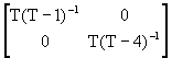
![]() +
+ ![]()
![]()
hence
![]() =
=![]() +
+ 
![]()
![]() =
= ![]()
![]() =
= ![]() .
.
AR(3)
![]() =
= +
+ 
![]()
+ 
![]()
Hence:
![]() =
=![]() +
+ 
![]()
![]() =
= ![]() [1 + 2
[1 + 2![]() ]
]
![]() =
= ![]() [
[![]() –
– ![]() – 2
– 2![]()
![]() ]
]
![]() =
= ![]()
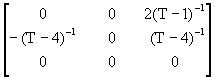
AR(4)
![]() =
=  +
+ 
![]()
+ 
![]()
![]() =
= ![]() +
+ 
![]()
Where:
![]()
![]()
![]() .
.
The non-zero elements of H are:
![]() ,
, ![]()
![]() ,
, ![]()
![]() ,
, ![]()
![]() ,
, ![]() ,
, ![]() ,
,
![]()
This representation defines t , ![]() and
and ![]() which can then be used in (12) to obtain the solution for
which can then be used in (12) to obtain the solution for ![]() in terms of
in terms of ![]() . Note that by reordering the
. Note that by reordering the ![]() vector as (
vector as (![]() ,
, ![]() ,
, ![]() ,
, ![]() , the recursive nature of the solution is apparent from the lower triangular nature of the resulting
, the recursive nature of the solution is apparent from the lower triangular nature of the resulting ![]() matrix.
matrix.
REFERENCES
Andrews, D. W. K. and Chen, H-Y. (1994), Approximately median-unbiased estimation of autoregressive models, Journal of Business and Economic Statistics, 12, 187-204.
Bhansali, R. J. (1981), Effects of not knowing the order of an autoregressive process on the mean squared error of prediction – I, Journal of the American Statistical Association, 76, 588-597.
Cordeiro, G. M. and Klein, R. (1994), Bias correction inARMA models, Statistics and Probability Letters, 19, 169-176.
Kendall, M. G. (1954), Note on the bias in the estimation of autocorrelation, Biometrika, 41, 403-404.
Kunitomo, N. and Yamamoto, T. (1985), Properties of predictors in misspecified autoregressive time series models, Journal of the American Statistical Association, 80, 941-950.
Marriott, F. H. C. and Pope, J. A. (1954), Bias in the estimation of autocorrelations, Biometrika, 41, 393-403.
Nelson, C. R. and Plosser, C. I. (1982), Trends and random walks in macroeconomic time series, Journal of Monetary Economics, 10, 129-162.
Orcutt, G. H. and Winokur, H. S. (1969), First order autoregression: inference, estimation, and prediction, Econometrica, 37, 1-14.
Pantula, S. G. and Fuller. W. A. (1985), Mean estimation bias in least squares estimation of autoregressive processes, Journal of Econometrics, 27, 99-121.
Rao, C. R. (1973), Linear Statistical Inference and its Applications, 2nd edition, John Wiley, New York.
Rudebusch, G. D. (1992), Trends and random walks in macroeconomic time series: a reexamination, International Economic Review, 33, 661-680.
Schotman, P. and van Dijk, H. K. (1991), On Bayesian routes to unit roots, Journal of Applied Econometrics, 6, 387-401.
Shaman, P. and Stine. R. A. (1988), The bias of autoregressive coefficient estimators, Journal of the American Statistical Association, 83, 842-848.
Stine, R. A. and Shaman, P. (1989), A fixed point characterisation for bias of autoregressive estimators, The Annals of Statistics, 17, 1275-1284.
Tanaka, K. (1984), An asymptotic expansion associated with the maximum likelihood estimators in ARMA models, Journal of the Royal Statistical Society, Series B, 46, 58-67.
Tjøstheim, D. and Paulsen, J. (1983), Bias of some common time series estimates, Biometrika, 70, 389-399.
Yamamoto, T. and Kunitomo, N. (1984), Asymptotic bias of the least squares estimator for multivariate autoregressive models, Journal of the Institute of Statistical mathematics, 36, 419-430.